Getting Started
rcfdtdpy can be installed into an Anaconda 3.6 environment via
conda install -c jr137 rcfdtdpy
or using pip via
pip install rcfdtdpy
From here it is easy to start one’s first simulation. Perhaps we want to simulate a terahertz spectroscopy conductivity
measurement of a Drude metal using the NumericMaterial class. We must first import the required libraries and
define our simulation parameters.
# Imports
from rcfdtdpy import Simulation, Current, NumericMaterial
import numpy as np
from scipy.fftpack import fft, fftfreq
from scipy.optimize import curve_fit
from matplotlib import pyplot as plt

# Speed of light
c0 = 3e8  # m/s
# Spatial step size
di = 0.03e-6  # 0.03 um
# Temporal step size
dn = di / c0  # (0.03 um) / (3e8 m/s) = 0.1 fs
# Permittivity of free space
epsilon0 = 8.854187e-12
# Permeability of free space
mu0 = np.divide(1, np.multiply(epsilon0, np.square(c0)))
# Define simulation bounds
i0 = -1e-6  # -1 um
i1 = 1e-6  # 1 um
n0 = -0.5e-12  # -0.5 ps
n1 = 2.5e-12  # 2.5 ps
# Calculate simulation dimensions
ilen, nlen = Simulation.calc_dims(i0, i1, di, n0, n1, dn)
# Calculate arrays that provide the spatial and temporal value of each cell
z, t = Simulation.calc_arrays(i0, i1, di, n0, n1, dn)
We next need to define the current present in our simulation. We do this by defining the location of the current pulse and the time at which the center of the current pulse occurs and then determining the spatial and temporal indices at which these space and time values correspond to.
# Define current pulse location and time
thz_loc = -0.5e-6  # -0.5 um
thz_time = 0  # 0 fs
# Find the corresponding location and time indices
thz_loc_ind = np.argmin(np.abs(np.subtract(z, thz_loc)))
thz_time_ind = np.argmin(np.abs(np.subtract(t, thz_time)))
We will define the terahertz pulse time profile as the second derivative of a Gaussian with FWHM of 90fs. We define this pulse as follows
thzshape = np.append(np.diff(np.diff(np.exp(-(((t - thz_time)/90e-15) ** 2)))), [0, 0])
We can now create our Current object
thzpulse = Current(thz_loc_ind, 0, ilen, nlen, thzshape)
Note that the length of the thzshape Numpy array is the same as the length of the simulation in time
nlen. For this reason the starting spatial index of the Current object must be set to 0. However
the length of the thzshape Numpy array can be less then the length of the simulation in time. If the user is
worried about the Current object taking up too much space in memory they might choose to define thzshape
over a small number of indices and simply define its starting index in space and time.
We are now prepared to define our material. Like with the Current object we begin by defining the location and
spatial and temporal extent of our material. We specify that our material starts at location \(0\) nm and is
\(50\) nm thick.
# Set material length
material_length = 0.050e-6  # 50 nm
# Set locations
material_start = 0
material_end = material_start + material_length
# Find the corresponding location and time indices
material_ind_start = np.argmin(np.abs(np.subtract(z, material_start)))
material_ind_end = np.argmin(np.abs(np.subtract(z, material_end)))
# Determine matrix length in indices
material_ind_len = material_ind_end - material_ind_start
The electric susceptibility of a Drude metal in time is given by
If you have no idea where this definition of susceptibility comes from, read up on the Lorentz oscillator. It is very easy to implement this material into our simulation.
# Define constants
a = np.complex64(1e16)
gamma = np.complex64(1e12 * 2 * np.pi)

# Define electric susceptibility in time
def chi(t):
    return a*(1-np.exp(-2*gamma*t))

# Define the high frequency permittivity in time (simply a constant)
def inf_perm(t):
    return 1

# Create our material!
drude = NumericMaterial(di, dn, ilen, nlen, material_ind_start, material_ind_end, chi, inf_perm)

# Export the susceptibility of the material
drude_chi = drude.export_chi()
Now that \(\chi^m\) has been calculated for each simulation time step, we can check that our Drude material has the expected form of electric susceptibility in time. We plot the electric susceptibility versus time
plt.plot(t*1e12, drude_chi)
plt.xlabel('time [ps]')
plt.ylabel('$\chi(t)$')
plt.show()
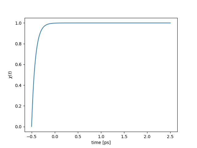
The analytic and simulated values of \(\chi(t)\) are in agreement. We must now specify what field values our simulation will record.
We would like to view our simulation evolving in time, meaning that we must store field values at each step in time. Lets say we would like to view the first third of the simulation.
nstore = np.arange(0, int(nlen/3), 100)
We choose to record the field values every 100 simulation steps for the first third of the simulation. We also would like to be able to calculate the transmission of our material in time. Therefore we wish to record the field value at every time step at the opposite side of the material from the current pulse. Since the material is \(50\) nm in length and starts at location \(0\) nm, recording the field value near the end of the simulation space will provide us with the transmitted field.
We specify that the simulation will have absorbing boundaries. The Simulation object is initialized and the
simulation is run.
s = Simulation(i0, i1, di, n0, n1, dn, epsilon0, mu0, 'absorbing', thzpulse, drude, nstore=nstore, istore=[ilen-6])
# Run simulation
s.simulate()
Now that the simulation has been run we export the fields stored by the Simulation object. The
Simulation object simulates two sets of electric and magnetic fields: a field that interacts with materials and
one that does not. This provides every simulation with a reference set of field values. We export the stored field
values as well as the electric electric susceptibility.
# Export field values
hfield, efield, hfield_ref, efield_ref = s.export_ifields()
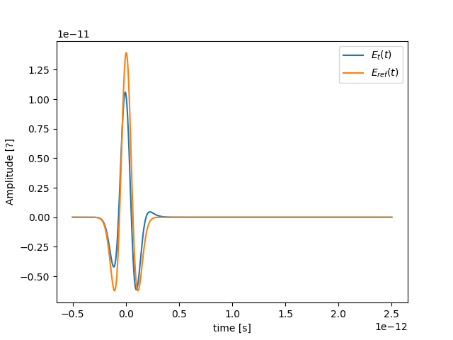
We proceed to produce plots of the transmitted and reference fields in time and frequency.
# Plot in time
plt.plot(t, np.real(efield), label='$E_{t}(t)$')
plt.plot(t, np.real(efield_ref), label='$E_{ref}(t)$')
plt.ylabel('Amplitude [?]')
plt.xlabel('time [s]')
plt.legend()
plt.show()
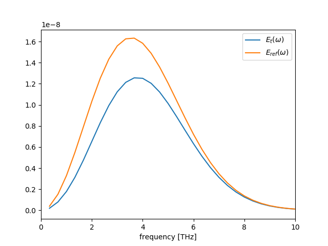
# Calculate time difference
dt = np.diff(t)[0] # Calculate time step difference in fs
# Calculate Fourier transforms
freq = fftfreq(nlen, dt) # in Hz
trans = fft(np.real(efield[:,0]))
ref = fft(np.real(efield_ref[:,0]))
# Remove unwanted frequencies
freq = freq[1:int(nlen/2)]
trans = trans[1:int(nlen/2)]
ref = ref[1:int(nlen/2)]
# Plot transformed fields
plt.plot(freq * 1e-12, np.abs(trans), label='$E_{t}(\omega)$')
plt.plot(freq * 1e-12, np.abs(ref), label='$E_{ref}(\omega)$')
plt.xlabel(r'frequency [THz]')
plt.xlim(0, 10)
plt.legend()
plt.show()
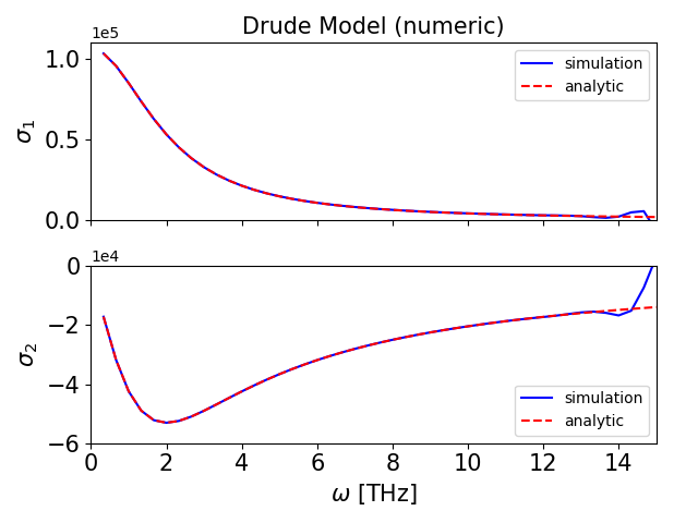
In the thin sample limit the conductivity of a material can be calculated via
where \(Z_0\) is the impedance of free space and \(t(\omega)=\frac{E_{t}(\omega)}{E_{ref}(\omega)}\). We next extract the conductivity of our simulated material and compare it to the analytical form of the conductivity of a Drude metal
# Remove zero indicies from all arrays
nonzero_ind = np.nonzero(ref)
freq = freq[nonzero_ind]
ref = ref[nonzero_ind]
trans = trans[nonzero_ind]

# Calculate t
spec = np.divide(trans, ref)

# Set constants
Z0 = np.multiply(mu0, c0) # Ohms (impedance of free space)

# Calculate the angular frequency
ang_freq = 2 * np.pi * freq # THz * 2pi

# Calculate conductivity
conductivity = np.multiply(np.divide(2, Z0*material_length), np.subtract(np.divide(1, spec), 1))

# Only fit to frequencies below 14THz, as the terahertz pulse has approximately zero amplitude above 14THz
freq_max = np.argmin(np.abs(np.subtract(14e12, freq)))

# Define fit functions
def cond_real(omega, sigma0, tau):
    return sigma0/(1+(tau*omega)**2)

def cond_imag(omega, sigma0, tau):
    return (-omega*tau*sigma0)/(1+(tau*omega)**2)

# Take real and imaginary parts
cfreq = freq[:freq_max]
creal = np.real(conductivity)[:freq_max]
cimag = np.imag(conductivity)[:freq_max]

# Run curve fit
popt_real, pcov_real = curve_fit(cond_real, cfreq, creal, p0=[1e5, 0.4e-12])
popt_imag, pcov_imag = curve_fit(cond_imag, cfreq, cimag, p0=[1e5, 0.2e-12])

fit_real = cond_real(freq, *popt_real)
fit_imag = cond_imag(freq, *popt_imag)

# Setup plot
fig, (ax0, ax1) = plt.subplots(2, 1, sharex=True, dpi=100)
ax0.set_ylabel(r'$\sigma_1$', fontsize=15)
ax1.set_ylabel(r'$\sigma_2$', fontsize=15)
ax1.set_xlabel(r'$\omega$ [THz]', fontsize=15)
ax0.set_title(r'Drude Model (numeric)', fontsize=15)
ax1.set_xlim(0, 15)
ax0.ticklabel_format(style='sci', scilimits=(0,0), axis='y')
ax0.tick_params(labelsize=15)
ax0.set_ylim(0, 1.1e5)
ax1.ticklabel_format(style='sci', scilimits=(0,0), axis='y')
ax1.tick_params(labelsize=15)
ax1.set_ylim(-6e4, 0)

# Plot simulated conductivity
ax0.plot(freq*1e-12, np.real(conductivity), 'b-', label='simulation')
ax1.plot(freq*1e-12, np.imag(conductivity), 'b-', label='simulation')

# Plot analytic conductivity
ax0.plot(freq*1e-12, fit_real, 'r--', label='analytic')
ax1.plot(freq*1e-12, fit_imag, 'r--', label='analytic')

ax0.legend()
ax1.legend()

plt.tight_layout()

plt.show()
That’s it! We have successfully simulated a Drude metal and examined how simulations are run with rcfdtdpy! You can
download the complete start.py file.